The behavior of the logistic map is shown in Cobweb plot form. The animation shows the change in behavior as the parameter (r in the figure) is increased from 1 to 4, starting from an initial function value of 0.2.
← ホームへ戻る
ロジスティック写像カオス理論分岐図周期倍分化ファイゲンバウム定数

ロジスティック写像単純な数式が導くカオスと秩序の世界

🗓 2026年8月11日

一見すると非常にシンプルな二次方程式が、予測不可能な「カオス」という複雑な挙動を生み出すことがあります。その代表例がロジスティック写像です。これは離散的な時間ステップで状態が変化する力学系であり、生物の個体数変動などのモデルとして利用されてきました。単純なルールからいかにして複雑性が生まれるのか、そのメカニズムを紐解いていきましょう。

ロジスティック写像は、以下の差分方程式によって定義されます。 xn+1 = r xn (1 - xn) ここで、xは0から1の間の値(例えば個体数比率)を、rは成長率などのパラメータを表します。この数式を繰り返し計算(反復)することで、次々と新しい値が生成され、その軌跡がシステムの挙動を決定します。
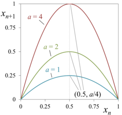
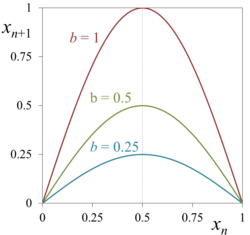
Graph of the logistic map (the relationship between x n + 1 {\displaystyle x_{n+1}} and x n {\displaystyle x_{n}} ). The graph has the shape of a parabola, and the vertex of the parabola changes as the parameter r changes.

Key Facts

  • 単純な構造: 1つの二次方程式の反復だけで、安定、周期振動、カオスという多様な状態を表現できる。
  • パラメータrの影響: rの値が変わることで、システムの挙動が劇的に変化する(分岐)。
  • 周期倍分化: 安定した状態から周期2、4、8…と周期が倍増していき、最終的にカオスへ至る。
  • 普遍性: このカオスへの道筋は、ロジスティック写像に限らず、多くの単峰型写像に共通して見られる。
  • 自己相似性: 分岐図を拡大すると、全体の構造と同じパターンが繰り返し現れるフラクタル構造を持つ。

システムの基礎と固定点

この写像において、変数を 0 ≤ x ≤ 1 の範囲に収めるためには、パラメータ r を 0 から 4 の間に設定する必要があります。rが4を超えると、計算結果が1を突き抜け、系が発散してしまいます。

システムが一定の値に落ち着く点を固定点と呼びます。ロジスティック写像には、x = 0 と x = 1 - 1/r という2つの固定点が存在します。これらの点が「安定」しているか「不安定」であるかは、その点における関数の傾き(微分係数)によって決まります。
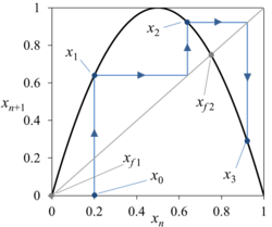
An example of a spider web projection of a trajectory on the graph of the logistic map, and the locations of the fixed points x f 1 {\displaystyle x_{f1}} and x f 2 {\displaystyle x_{f2}} on the graph.

挙動を視覚化する手法として、関数グラフと45度線を用いて軌跡を追う「クモの巣図(Cobweb plot)」が有効です。これにより、値が固定点に収束するのか、あるいは振動するのかを一目で理解できます。
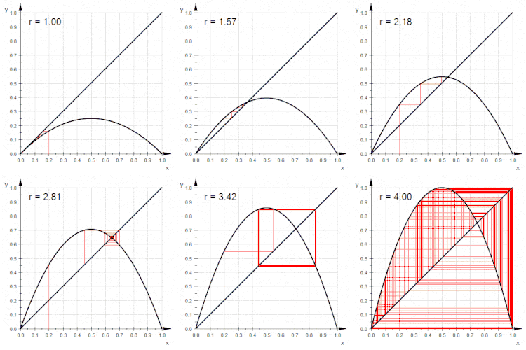
The behavior of the logistic map is shown in Cobweb plot form. The animation shows the change in behavior as the parameter (r in the figure) is increased from 1 to 4, starting from an initial function value of 0.2.

パラメータrによる挙動の変化

rの値を上げていくと、システムは段階的にその性質を変えていきます。

1. 絶滅と収束 (0 ≤ r < 3)

rが1未満の場合、どのような初期値から始めても最終的に x = 0 に収束します。これは生物学的には個体数が絶滅することを意味します。rが1を超えると、x = 0 は不安定になり、代わりに x = 1 - 1/r という正の固定点へ収束するようになります。
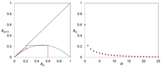
Spider plot (left) and time series (n vs. x n) (right) for parameter r = 0.9. The trajectory converges monotonically to 0.

Transcritical bifurcation of the logistic map occurring at r = 1. For r < 1, x f 2 {\displaystyle x_{f2}} exists outside [0, 1] as an unstable fixed point, but for r = 1, the two fixed points collide, and for r > 1, x f 2 {\displaystyle x_{f2}} appears between [0, 1] as a stable fixed point.

rが2から3の間になると、収束の仕方が変化します。単調に近づくのではなく、固定点の周りを振動しながら収束するようになります。
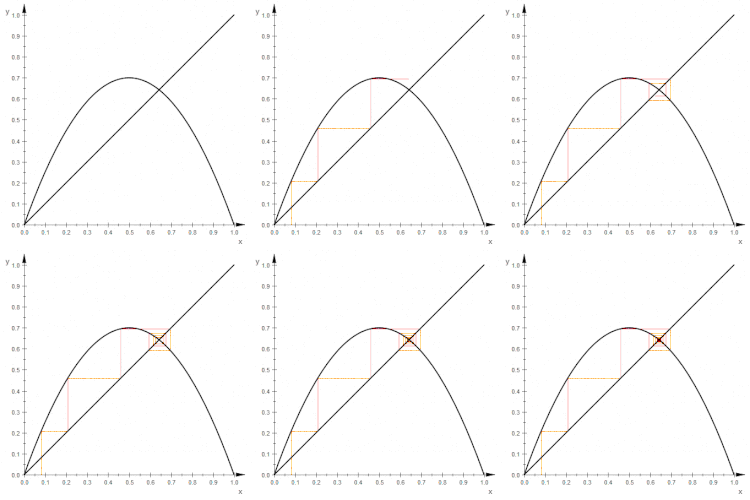
Animation of the spider projection at a = 2.8, converging around a fixed point.

2. 周期倍分化の始まり (3 ≤ r < 3.56995)

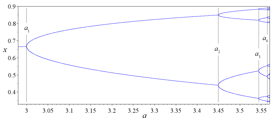
rが3を超えると、固定点は不安定になり、値が2つの値の間を行き来する「周期2」の振動が始まります。さらにrを大きくすると、周期4、周期8、周期16…と、安定した周期が倍々に増えていく周期倍分化(Period-doubling bifurcation)という現象が発生します。
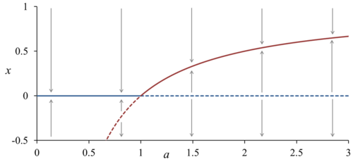
Bifurcation diagram of the logistic map for parameters 0 to 3. The blue line represents the fixed point x f 1 = 0 {\displaystyle x_{f1}=0} , and the red line represents the fixed point x f 2 = 1 − 1 / r {\displaystyle x_{f2}=1-1/r} Represents.

Bifurcation diagram of the period-doubling bifurcation cascade occurring between parameters r 1 = 3 {\displaystyle r_{1}=3} and a ∞ = 3.56994... {\displaystyle a_{\infty }=3.56994...} . After 64 periods ( a 5 {\displaystyle a_{5}} ), the spacing becomes very narrow and almost collapses.

3. カオス領域の出現 (3.56995 < r ≤ 4)

rが約3.56994(ファイゲンバウム点)を超えると、周期性は失われ、値は不規則に変動するカオス状態に入ります。しかし、カオス領域の中にも、突然安定した周期的な挙動に戻る「窓(Window)」と呼ばれる区間が存在します。例えば r ≈ 3.8284 付近では周期3の安定した軌道が現れます。
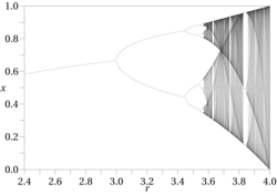
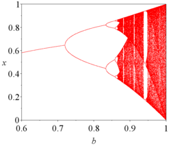
Bifurcation diagram for the logistic map. The attractor for any value of the parameter r is shown on the vertical line at that r.

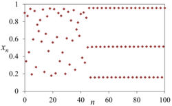
Transient chaos at a = 3.8285. The system behaves chaotically until it is attracted into a periodic 3 orbit.

カオスの深層:普遍性と自己相似性

ロジスティック写像の最も驚くべき点は、その構造が持つ普遍性(Universality)です。ミッチェル・ファイゲンバウムは、周期倍分化が起こる間隔の比率が、関数の具体的な形に関わらず一定の値(δ ≈ 4.6692)に収束することを発見しました。

{\displaystyle r}

また、このシステムは自己相似的な階層構造を持っています。分岐図の一部を拡大すると、元の分岐図とそっくりな構造が無限に繰り返されており、これはフラクタル幾何学的な性質を示しています。
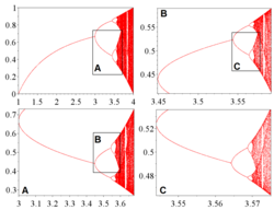
Self-similar hierarchical structure of the entire trajectory map of the logistic map

Self-similar hierarchical structure of windows of the logistic map

r = 4 のとき、系は完全にカオス的になります。この状態では、初期値のわずかな違いが時間とともに指数関数的に拡大するため、長期的な予測が不可能になります。しかし、統計的な分布(不変測度)を調べると、特定の密度関数に従っていることがわかります。
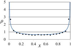
Graph of the invariant measure ρ(x) for r = 4. The dot plot shows the actual frequency of points obtained over 10,000 iterations (with height scaled to ρ (x)).

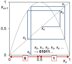
If the orbit of the logistic map f r = 4 {\displaystyle f_{r=4}} is converted into a string of 0s and 1s, any string of symbols can be reproduced.

応用と拡張

ロジスティック写像の概念は、単なる数学的興味に留まらず、様々な分野に応用されています。

  • 人口動態モデル: 環境収容力を持つ個体数の変動をシミュレーションする。
  • 擬似乱数生成: カオス的な不規則性を利用して、予測困難な乱数を生成する。
  • 複素数への拡張: 変数を複素数に広げると、有名なマンデルブロ集合の構造と深く関連します。

Correspondence between the orbit diagram of a variation of the logistic map (top) and the Mandelbrot set (bottom)

また、複数の写像を結合させた「結合写像格子」などのモデルでは、カオス状態にある個々の要素が同期したり、複雑なパターンを形成したりする現象が研究されています。
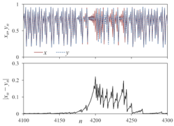
Changes in two variables (top) and their difference (bottom) in the coupled map model ( 6-2 ) with a = 3.8 and D = 0.43 . The two variables suddenly become out of sync after synchronization, and then return to the sync state.

まとめ:ロジスティック写像の特性

以下に、パラメータrの変化に伴うシステムの挙動をまとめます。

ロジスティック写像のパラメータrと挙動の対応表
パラメータ r の範囲 主な挙動 状態の特性
0 ≤ r < 1 0への収束 個体数の絶滅
1 ≤ r < 3 正の固定点への収束 安定した平衡状態
3 ≤ r < 3.449 周期2の振動 2つの値の間を交互に移動
3.449 ≤ r < 3.57 周期倍分化 周期 4, 8, 16... と倍増
3.57 ≤ r ≤ 4 カオス 不規則な変動(一部に周期窓あり)

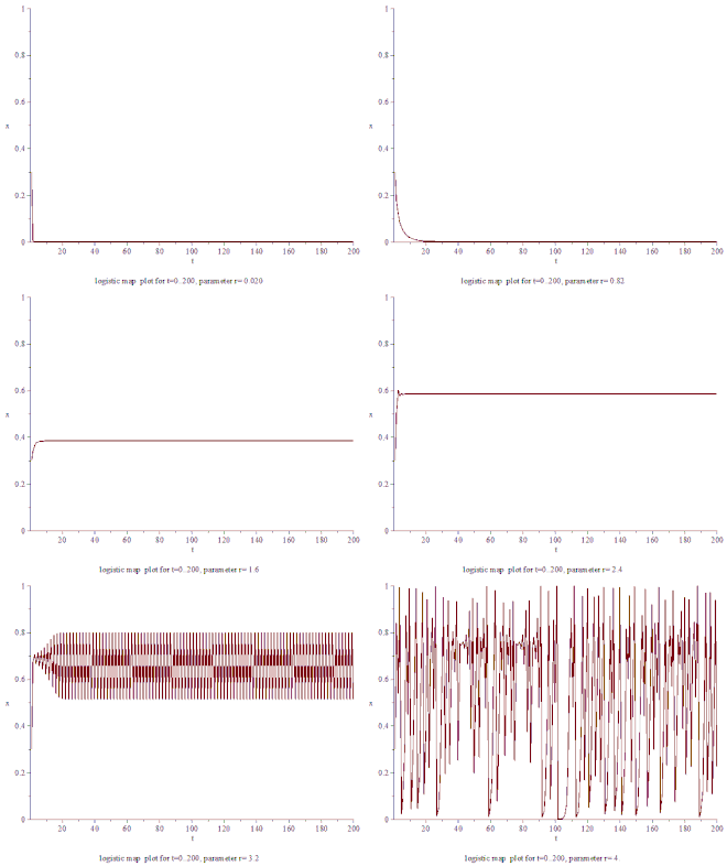
The sequence behaviour from r=0.02 to r=4, one can visualize the horizontal coordinate as time, and the vertical coordinate either as a position in space at time t or as the population size at time t

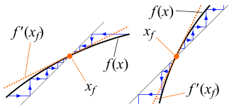
Tangent slopes of an asymptotically stable fixed point (left) and an unstable fixed point (right) and the state of the surrounding orbits

An example of the construction of a Cantor set: if you keep removing the central third of a line segment infinitely, you will end up with a shape that appears to have zero length but has an uncountably infinite number of points, each of which has an infinitesimal neighborhood of other points.

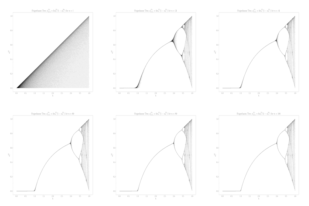
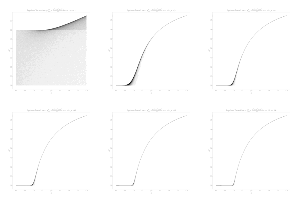
Evolution of different initial conditions as a function of r (The parameter k from the figure corresponds to the parameter r from the definition in the article.)

Evolution of different initial conditions as a function of r with bias (The parameter k from the figure corresponds to the parameter r from the definition in the article.)

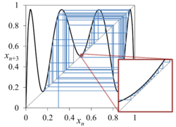
Channel patterns appearing in the graph of f3 (x)

For the logistic map with r = 4.5, trajectories starting from almost any point in [0, 1] go towards minus infinity.

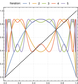
Logistic function f (blue) and its iterated versions f2, f3, f4 and f5 for r = 3.5. For example, for any initial value on the horizontal axis, f4 gives the value of the iterate four iterations later.

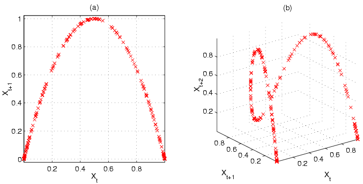
Two- and three-dimensional Poincaré plots show the stretching-and-folding structure of the logistic map

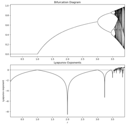
Logistic map with Lyapunov exponent function

Graph of the sine map ( 4-1 )

Orbit diagram of the sine map ( 4-1 )

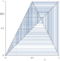
Orbital view of the tent map ( 4-8 ). It has a topological conjugate relationship with the a = 4 logistic map.

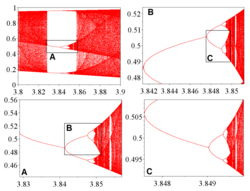
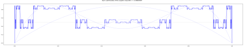
At the point of chaos r ∗ = 3.5699 ⋯ {\displaystyle r^{*}=3.5699\cdots } , as the period-doublings f r ∗ 1 , f r ∗ 2 , f r ∗ 4 , f r ∗ 8 , f r ∗ 16 , … {\displaystyle f_{r^{*}}^{1},f_{r^{*}}^{2},f_{r^{*}}^{4},f_{r^{*}}^{8},f_{r^{*}}^{16},\dots } are repeated, the graphs seem to resemble each other, except that they are shrunken towards the middle, and rotated by 180 degrees, converging to a fractal.

{\displaystyle \alpha }

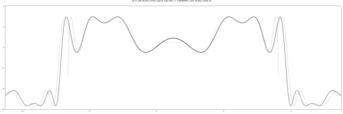
At the point of chaos r ∗ = 3.5699 ⋯ {\displaystyle r^{*}=3.5699\cdots } , as the functional equation iteration f ( x ) ↦ − α f ( f ( − x / α ) ) {\displaystyle f(x)\mapsto -\alpha f(f(-x/\alpha ))} with α = 2.5029 … {\displaystyle \alpha =2.5029\dots } is repeated, the map does converge to a limit.

{\displaystyle f_{r}^{\infty }}

{\displaystyle r^{*}=3.84943\dots }

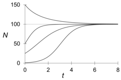
An example of a solution to the logistic equation. After time t, the population size N converges to the carrying capacity K regardless of the initial value.

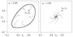
The trajectory of the delayed logistic map. The initial values ( x 0 , y 0 ) {\displaystyle (x_{0},y_{0})} are the same in both figures, but at the bifurcation point r = 2, the trajectory is attracted to a closed curve (left) and a point (right).

Stanislaw Ulam

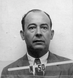
John von Neumann

Robert May (photographed in 2009)

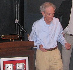
Mitchell Feigenbaum (photographed in 2006)

Frequently Asked Questions

ロジスティック写像でいう「カオス」とは具体的にどのような状態ですか?

決定論的な数式に基づいているため、次の値は完全に決まっていますが、挙動が極めて不規則で、初期値のわずかな差が時間とともに劇的に拡大するため、長期的な予測が実質的に不可能な状態を指します。

なぜ周期が「倍」に増えていくのですか?

これは「周期倍分化」と呼ばれる現象で、ある周期の固定点が不安定になると、その周囲に新しい安定した周期(元の2倍の長さ)の軌道が生まれるためです。これは多くの非線形システムに見られる普遍的なルートです。

r = 4 のとき、値は完全にランダムになるのでしょうか?

見た目はランダムに見えますが、実際には決定論的なルールに従っています。ただし、統計的な分布(不変測度)を持っており、特定の範囲に値が現れやすいという構造を持っています。

このモデルは実際の生物の個体数予測に使えるのでしょうか?

単純化されたモデルであるため、そのまま正確な予測に使うことは困難です。しかし、「環境の限界がある中で個体数が変動する」という基本的なメカニズムや、ある条件下で個体数が激しく変動しうることを理解するための強力な理論的枠組みを提供しています。

ファイゲンバウム定数とは何ですか?

周期倍分化が起こるパラメータの間隔が、回数を重ねるごとに一定の比率で縮まっていくことを示す定数(δ ≈ 4.6692)です。この値はロジスティック写像だけでなく、同様の性質を持つ多くの関数で共通して現れます。

References

  1. Lorenz, Edward N. (1964-02-01). "The problem of deducing the climate from the governing equations". Tellus. 16 (1): 1–11. :1964Tell...16....1L. :10.3402/tellusa.v16i1.8893.  0040-2826.
  2. "Logistic Equation". .
  3. See .
  4. Gleick, James (1987). Chaos: Making a New Science. London: Penguin Books.  .
  5. (2004). Fractals and Chaos, The Mandelbrot Set and Beyond. pp. 259–267. :10.1007/978-1-4757-4017-2.  .
  6. Tsuchiya, Takashi; Yamagishi, Daisuke (February 11, 1997). "The Complete Bifurcation Diagram for the Logistic Map". Z. Naturforsch. 52a (6–7): 513–516. :1997ZNatA..52..513T. :10.1515/zna-1997-6-708.  101491730.
  7. Bonet, J.; Martínez-Giménez, F.; Peris, A. (2001). "A Banach space which admits no chaotic operator". Bulletin of the London Mathematical Society. 33 (2): 196–198. :10.1112/blms/33.2.196.  121429354.
  8. Zhang, Cheng (October 2010). "Period three begins". . 83 (4): 295–297. :10.4169/002557010x521859.  123124113.
  9. Bechhoefer, John (1996-04-01). "The Birth of Period 3, Revisited". Mathematics Magazine. 69 (2): 115–118. :10.1080/0025570X.1996.11996402.  0025-570X.
  10. Jeffries, Carson; Pérez, José (1982). "Observation of a Pomeau–Manneville intermittent route to chaos in a nonlinear oscillator". . 26 (4): 2117–2122. :1982PhRvA..26.2117J. :10.1103/PhysRevA.26.2117.  119466337.

📸 フォトギャラリー

The behavior of the logistic map is shown in Cobweb plot form. The animation shows the change in behavior as the parameter (r in the figure) is increased from 1 to 4, starting from an initial function value of 0.2.
The sequence behaviour from r=0.02 to r=4, one can visualize the horizontal coordinate as time, and the vertical coordinate either as a position in space at time t or as the population size at time t
Graph of the logistic map (the relationship between x n + 1 {\displaystyle x_{n+1}} and x n {\displaystyle x_{n}} ). The graph has the shape of a parabola, and the vertex of the parabola changes as the parameter r changes.
An example of a spider web projection of a trajectory on the graph of the logistic map, and the locations of the fixed points x f 1 {\displaystyle x_{f1}} and x f 2 {\displaystyle x_{f2}} on the graph.
Spider plot (left) and time series (n vs. x n) (right) for parameter r = 0.9. The trajectory converges monotonically to 0.
Tangent slopes of an asymptotically stable fixed point (left) and an unstable fixed point (right) and the state of the surrounding orbits
Transcritical bifurcation of the logistic map occurring at r = 1. For r < 1, x f 2 {\displaystyle x_{f2}} exists outside [0, 1] as an unstable fixed point, but for r = 1, the two fixed points collide, and for r > 1, x f 2 {\displaystyle x_{f2}} appears between [0, 1] as a stable fixed point.
Animation of the spider projection at a = 2.8, converging around a fixed point.
Bifurcation diagram of the logistic map for parameters 0 to 3. The blue line represents the fixed point x f 1 = 0 {\displaystyle x_{f1}=0} , and the red line represents the fixed point x f 2 = 1 − 1 / r {\displaystyle x_{f2}=1-1/r} Represents.
Bifurcation diagram of the period-doubling bifurcation cascade occurring between parameters r 1 = 3 {\displaystyle r_{1}=3} and a ∞ = 3.56994... {\displaystyle a_{\infty }=3.56994...} . After 64 periods ( a 5 {\displaystyle a_{5}} ), the spacing becomes very narrow and almost collapses.
An example of the construction of a Cantor set: if you keep removing the central third of a line segment infinitely, you will end up with a shape that appears to have zero length but has an uncountably infinite number of points, each of which has an infinitesimal neighborhood of other points.
Evolution of different initial conditions as a function of r (The parameter k from the figure corresponds to the parameter r from the definition in the article.)
Evolution of different initial conditions as a function of r with bias (The parameter k from the figure corresponds to the parameter r from the definition in the article.)
Bifurcation diagram for the logistic map. The attractor for any value of the parameter r is shown on the vertical line at that r.
Transient chaos at a = 3.8285. The system behaves chaotically until it is attracted into a periodic 3 orbit.
Channel patterns appearing in the graph of f3 (x)
Self-similar hierarchical structure of the entire trajectory map of the logistic map
Self-similar hierarchical structure of windows of the logistic map
Graph of the invariant measure ρ(x) for r = 4. The dot plot shows the actual frequency of points obtained over 10,000 iterations (with height scaled to ρ (x)).
If the orbit of the logistic map f r = 4 {\displaystyle f_{r=4}} is converted into a string of 0s and 1s, any string of symbols can be reproduced.
For the logistic map with r = 4.5, trajectories starting from almost any point in [0, 1] go towards minus infinity.
Logistic function f (blue) and its iterated versions f2, f3, f4 and f5 for r = 3.5. For example, for any initial value on the horizontal axis, f4 gives the value of the iterate four iterations later.
Two- and three-dimensional Poincaré plots show the stretching-and-folding structure of the logistic map
Logistic map with Lyapunov exponent function
Graph of the sine map ( 4-1 )
Orbit diagram of the sine map ( 4-1 )
Orbital view of the tent map ( 4-8 ). It has a topological conjugate relationship with the a = 4 logistic map.
{\displaystyle r}
At the point of chaos r ∗ = 3.5699 ⋯ {\displaystyle r^{*}=3.5699\cdots } , as the period-doublings f r ∗ 1 , f r ∗ 2 , f r ∗ 4 , f r ∗ 8 , f r ∗ 16 , … {\displaystyle f_{r^{*}}^{1},f_{r^{*}}^{2},f_{r^{*}}^{4},f_{r^{*}}^{8},f_{r^{*}}^{16},\dots } are repeated, the graphs seem to resemble each other, except that they are shrunken towards the middle, and rotated by 180 degrees, converging to a fractal.
{\displaystyle \alpha }
At the point of chaos r ∗ = 3.5699 ⋯ {\displaystyle r^{*}=3.5699\cdots } , as the functional equation iteration f ( x ) ↦ − α f ( f ( − x / α ) ) {\displaystyle f(x)\mapsto -\alpha f(f(-x/\alpha ))} with α = 2.5029 … {\displaystyle \alpha =2.5029\dots } is repeated, the map does converge to a limit.
{\displaystyle f_{r}^{\infty }}
{\displaystyle r^{*}=3.84943\dots }
An example of a solution to the logistic equation. After time t, the population size N converges to the carrying capacity K regardless of the initial value.
Changes in two variables (top) and their difference (bottom) in the coupled map model ( 6-2 ) with a = 3.8 and D = 0.43 . The two variables suddenly become out of sync after synchronization, and then return to the sync state.
Correspondence between the orbit diagram of a variation of the logistic map (top) and the Mandelbrot set (bottom)
The trajectory of the delayed logistic map. The initial values ( x 0 , y 0 ) {\displaystyle (x_{0},y_{0})} are the same in both figures, but at the bifurcation point r = 2, the trajectory is attracted to a closed curve (left) and a point (right).
Stanislaw Ulam
John von Neumann
Robert May (photographed in 2009)
Mitchell Feigenbaum (photographed in 2006)