自然界や社会現象における複雑な変化を数学的に扱う「力学系」という分野において、アトラクタ(Attractor)は極めて重要な概念です。簡単に言えば、システムが時間の経過とともに最終的にたどり着く「安定した状態の集合」のことを指します。初期状態が多少異なっていても、多くのケースでシステムは特定のパターンや値へと引き寄せられます。この「引き寄せる」性質こそがアトラクタの正体です。
例えば、摩擦のある場所で振り子を揺らすと、最終的には最下点で静止します。この「最下点」という状態が、このシステムにおけるアトラクタです。物理的な座標だけでなく、経済学におけるインフレ率や失業率といった変数など、多次元的なデータセットにおいても同様の概念が適用されます。
![Visual representation of a strange attractor.[1] Another visualization of the same 3D attractor is this video. Code capable of rendering this is available.](/images/1f/70/1f709e9b1603b004cc6241cb1317bd8062eb7d9741382459b56715987c8b94d7.jpg)
Key Facts
- 定義: システムが多様な初期条件から進化し、最終的に収束する状態の集合。
- 安定性: アトラクタ近傍に達したシステムは、わずかな乱れがあってもその付近に留まり続ける。
- 種類: 単純な「点」や「周期的な軌道」から、複雑な「フラクタル構造」を持つものまで存在する。
- 吸引領域: あるアトラクタに最終的に吸収される初期状態の範囲を「吸引領域(Basin of Attraction)」と呼ぶ。
- カオスとの関係: ストレンジアトラクタを持つシステムは、局所的に不安定(初期値鋭敏性)ながら、全体としては安定した構造を持つ。
アトラクタの数学的構造と定義
数学的に見ると、アトラクタは相空間(システムのすべての可能な状態を座標として表した空間)の中のサブセットとして定義されます。ある状態 $a$ が時間 $t$ とともにどのように変化するかを関数 $f(t, a)$ で表したとき、アトラクタ $A$ は以下の条件を満たす領域となります。
- 前方不変性: 一度アトラクタ $A$ に入った状態は、その後もずっと $A$ の中に留まり続ける。
- 吸引領域の存在: $A$ の周囲に、時間の経過とともに必ず $A$ へと収束する点(初期値)の集合 $B(A)$ が存在する。
- 最小性: $A$ の内部に、上記2つの条件を同時に満たすさらに小さな部分集合が存在しない。
この概念は、単なる「極限集合」とは異なります。極限集合の中には、わずかな摂動(乱れ)によってシステムがその領域から永久に離れてしまう不安定なものもありますが、アトラクタは周囲から状態を引き寄せ、保持する性質を持っています。
アトラクタの主な種類
固定点(Fixed Point)
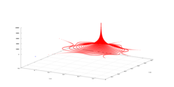
最も単純な形式で、システムが単一の点に収束する場合です。例えば、ボウルの中を転がるボールが底で止まる状態や、減衰振動する振り子が静止する状態がこれにあたります。逆に、逆さまのボウルに置かれたボールは、静止していれば「固定点」ですが、少しでも動けば離れていくため、アトラクタではなく「リペラー(反発点)」と呼ばれます。
周期的なアトラクタ:リミットサイクルと有限点
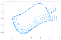
システムが一定のパターンを繰り返す場合です。離散時間システムでは、いくつかの点が順番に訪問される「周期点」の集合となります。連続時間システムでは、孤立した閉軌道であるリミットサイクルとして現れます。心拍や時計の振り子(エネルギー供給がある場合)などが代表例です。
リミットトーラス
複数の異なる周波数が共存し、それらが無理数比(不整合)である場合、軌道は閉じず、ドーナツ状の構造である「トーラス」を形成します。これを $N$ 個の不整合な周波数を持つ場合に $N$-トーラスと呼びます。
ストレンジアトラクタ(Strange Attractor)
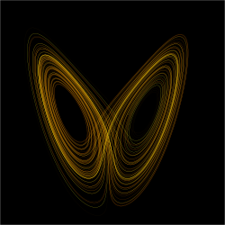
幾何学的に単純な点や線で記述できず、フラクタル構造(非整数次元のハウスドルフ次元)を持つアトラクタです。多くの場合、ここでの挙動は「カオス的」です。つまり、アトラクタ上の非常に近い2点が時間とともに指数関数的に離れていく「初期値鋭敏性」を持ちながら、システム全体としてはアトラクタの範囲内に留まり続けます。
システムの進化とパラメータの影響
システムがどのようなアトラクタを持つかは、そのシステムを規定するパラメータによって劇的に変化します。有名な例がロジスティック写像です。パラメータ $r$ の値を変えると、アトラクタは単一の点から、2点、4点へと分かれ(周期倍分枝)、最終的には無限の点からなるカオス的な状態へと移行します。
![Bifurcation diagram of the logistic map. The attractor(s) for values of the parameter r {\displaystyle r} from [ 2.4 , 4 ] {\displaystyle [2.4,4]} are shown on the vertical axis for 0 < x < 1 {\displaystyle 0<x<1} . The colour of a point indicates how often the point ( r , x ) {\displaystyle (r,x)} is visited over the course of 106 iterations: frequently encountered values are coloured in blue, less frequently encountered values are yellow. A bifurcation occurs around r ≈ 3.0 {\displaystyle r\approx 3.0} , a second bifurcation (leading to four attractor values) is seen around r ≈ 3.5 {\displaystyle r\approx 3.5} . The dynamics become increasingly complicated for r > 3.6 {\displaystyle r>3.6} , interspersed with regions of simpler behaviour (white stripes).](/images/21/dd/21dd6f7b6909ca9e43a3b6508cfb35b5d788638b6486f6d417fe1ca0ef6a0478.webp)
吸引領域の複雑性
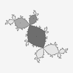
非線形システムでは、どの初期値がどのアトラクタに向かうかを示す「吸引領域」が非常に複雑になることがあります。例えば、ニュートン法を用いて方程式の根を求める際、開始点によってどの根に収束するかが決定されますが、その境界はフラクタル状に複雑に絡み合っていることがあります。
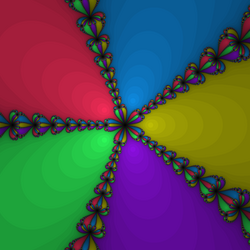
アトラクタの特性まとめ
| 種類 | 幾何学的形状 | 挙動の特性 | 具体例 |
|---|---|---|---|
| 固定点 | 点 | 静止・収束 | 摩擦のある振り子の停止状態 |
| リミットサイクル | 閉曲線(ループ) | 定期的・周期的 | 安静時の心拍 |
| リミットトーラス | トーラス(円環面) | 準周期的 | 不整合な周波数を持つ惑星軌道 |
| ストレンジアトラクタ | フラクタル | カオス的・非周期的 | ローレンツ・アトラクタ(気象モデル) |
Frequently Asked Questions
アトラクタとリペラーの違いは何ですか?
アトラクタは周囲の状態を自分の方へ引き寄せ、そこに留まらせる性質を持ちますが、リペラー(反発点)は逆に周囲の状態を遠ざける性質を持ちます。どちらも不変集合ですが、安定性が正反対です。
ストレンジアトラクタは常にカオス的ですか?
多くの場合、ストレンジアトラクタ上のダイナミクスはカオス的ですが、数学的には「ストレンジ(フラクタル構造を持つ)だが非カオス的」なアトラクタも存在します。
吸引領域(Basin of Attraction)とは具体的に何を指しますか?
ある特定のアトラクタに最終的に到達するすべての初期状態の集合のことです。線形システムでは相空間全体が一つの吸引領域になることが多いですが、非線形システムでは複数のアトラクタが存在し、領域が複雑に分断されていることがあります。
なぜストレンジアトラクタは予測が難しいのですか?
ストレンジアトラクタ上の軌道は「初期値鋭敏性」を持っているためです。たとえ極めて小さな測定誤差があっても、時間の経過とともにその差が指数関数的に拡大するため、長期的な状態予測が事実上不可能になります。
物理的なシステム以外にアトラクタの概念は使われますか?
はい。経済学における変数(インフレ率と失業率など)の変動や、生物学における個体数変動モデル、さらには偏微分方程式を用いた流体力学(ナビエ・ストークス方程式など)の解析にも利用されています。
References
- Desprez, Nicolas. "Chaoscope > Gallery". www.chaoscope.org. Archived from the original on 30 September 2023. Retrieved 21 December 2024.
- "Attractor". . Retrieved 30 May 2021.
- Carvalho, A.; Langa, J.A.; Robinson, J. (2012). Attractors for infinite-dimensional non-autonomous dynamical systems. Vol. 182. Springer. p. 109.
- Kantz, H.; Schreiber, T. (2004). Nonlinear time series analysis. Cambridge university press.
- (1985). "On the concept of attractor". Communications in Mathematical Physics. 99 (2): 177–195. :1985CMaPh..99..177M. :10.1007/BF01212280. 120688149.
- Greenwood, J. A.; J. B. P. Williamson (6 December 1966). "Contact of Nominally Flat Surfaces". Proceedings of the Royal Society. 295 (1442): 300–319. :1966RSPSA.295..300G. :10.1098/rspa.1966.0242. 137430238.
- Vorberger, T. V. (1990). Surface Finish Metrology Tutorial (PDF). U.S. Department of Commerce, National Institute of Standards (NIST). p. 5.
- Grebogi Celso, Ott Edward, Yorke James A (1987). "Chaos, Strange Attractors, and Fractal Basin Boundaries in Nonlinear Dynamics". Science. 238 (4827): 632–638. :1987Sci...238..632G. :10.1126/science.238.4827.632. 17816542. 1586349.
{{}}: CS1 maint: multiple names: authors list () - Ruelle, David; Takens, Floris (1971). "On the nature of turbulence". Communications in Mathematical Physics. 20 (3): 167–192. :1971CMaPh..20..167R. :10.1007/bf01646553. 17074317.
- Chekroun M. D.; Simonnet E. & (2011). "Stochastic climate dynamics: Random attractors and time-dependent invariant measures". Physica D. 240 (21): 1685–1700. :2011PhyD..240.1685C. 10.1.1.156.5891. :10.1016/j.physd.2011.06.005.
{{}}: Cite uses deprecated parameter|citeseerx=()
📸 フォトギャラリー