一見すると完全にランダムで無秩序に見える現象の中にも、実は厳格な数学的法則やパターンが隠れていることがあります。これを研究するのがカオス理論です。この理論は、単純な決定論的な法則に従いながらも、極めて複雑で予測不可能な挙動を示す「動的システム」に焦点を当てています。
かつて、不規則な変動は単なる「乱数」や「ノイズ」として片付けられてきました。しかし、カオス理論は、その見かけ上の混乱の中に、自己相似性やフィードバックループ、そして自己組織化といった深い構造が存在することを明らかにしました。
Key Facts
- 決定論的カオス:未来の状態が現在の状態で完全に決まっているにもかかわらず、長期的な予測が不可能な状態を指します。
- 初期値鋭敏性:開始時のごくわずかな差が、時間の経過とともに劇的な結果の違いを生む特性です。
- バタフライ効果:ブラジルの蝶の羽ばたきがテキサスで竜巻を引き起こすかもしれないという比喩で、小さな変化が連鎖的に巨大な影響を及ぼすことを示します。
- ストレンジアトラクター:カオス的なシステムが時間とともに収束していく、複雑でフラクタルな構造を持つ軌道のことです。
カオスの本質:なぜ予測できないのか
カオス理論の核心は、「決定論的であること」と「予測可能であること」は別物であるという点にあります。決定論的なシステムとは、ランダムな要素を含まず、現在の状態から次の状態が一意に決まるシステムを指します。しかし、非線形なシステムにおいては、測定誤差や計算上の丸め誤差のような極めて小さな差異が、指数関数的に増幅されます。
気象学者のエドワード・ローレンツは、この現象を「現在は未来を決定するが、近似的な現在は近似的な未来を決定しない」と表現しました。つまり、現在の状態を100%正確に把握できない限り、十分な時間が経過した後の未来を予測することは理論的に不可能なのです。
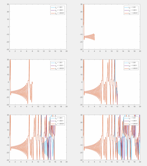
初期値への鋭敏な依存性
この特性は、物理的なシステムにおいて顕著に現れます。例えば、二重振り子は非常にシンプルな構造ですが、開始角度をわずかに変えるだけで、その後の軌道は全く異なるものになります。これは、単純な物理法則に従っていても、結果がカオス的になる典型例です。
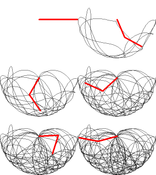
カオスを形作る数学的メカニズム
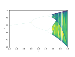
ロジスティック写像と分岐
カオスの発生を理解するための代表的なモデルに「ロジスティック写像」があります。これは個体数変動などのモデル化に用いられる単純な数式ですが、パラメータ(成長率など)を変化させると、安定した状態から周期的な変動へ、そして最終的にカオス状態へと移行します。この過程を視覚化したものが分岐図であり、周期倍増という現象を経てカオスへと至る様子が分かります。
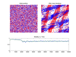
また、このような写像を繰り返すと、初期状態の点集合が空間全体に複雑に散らばる「トポロジカル混合」という現象が起こります。これにより、システム内の状態が均一に混ざり合い、不可逆的な拡散が生じます。
![Six iterations of a set of states [ x , y ] {\displaystyle [x,y]} passed through the logistic map. The first iterate (blue) is the initial condition, which essentially forms a circle. Animation shows the first to the sixth iteration of the circular initial conditions. It can be seen that mixing occurs as we progress in iterations. The sixth iteration shows that the points are almost completely scattered in the phase space. Had we progressed further in iterations, the mixing would have been homogeneous and irreversible. The logistic map has equation x k + 1 = 4 x k ( 1 − x k ) {\displaystyle x_{k+1}=4x_{k}(1-x_{k})} . To expand the state-space of the logistic map into two dimensions, a second state, y {\displaystyle y} , was created as y k + 1 = x k + y k {\displaystyle y_{k+1}=x_{k}+y_{k}} , if x k + y k < 1 {\displaystyle x_{k}+y_{k}<1} and y k + 1 = x k + y k − 1 {\displaystyle y_{k+1}=x_{k}+y_{k}-1} otherwise.](/images/3f/19/3f19b24150dad88342fdfa7cc4947880f7bbc786f098f0b75df4ca68ff8aa7f4.gif)
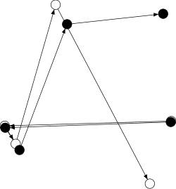
ストレンジアトラクターの構造
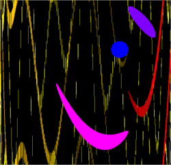
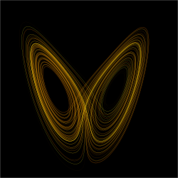
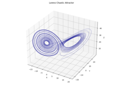
カオス的なシステムを相空間(状態を座標として表した空間)で観察すると、軌道はある特定の領域に引き寄せられます。この引き寄せられる領域をアトラクターと呼びますが、カオス系におけるそれは、決して同じ点を繰り返さず、かつ複雑な層状構造を持つ「ストレンジアトラクター」となります。ローレンツ・アトラクターは、その代表例として知られる蝶のような形状の軌道です。
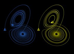
興味深いことに、あるシステムの中にはカオス的な軌道と、安定した非カオス的な軌道が共存している場合があります。初期値によって、システムがどちらの領域に引き寄せられるかが決まります。
![Coexisting chaotic and non-chaotic attractors within the generalized Lorenz model.[37][38][39] There are 128 orbits in different colors, beginning with different initial conditions for dimensionless time between 0.625 and 5 and a heating parameter r = 680. Chaotic orbits recurrently return close to the saddle point at the origin. Nonchaotic orbits eventually approach one of two stable critical points, as shown with large blue dots. Chaotic and nonchaotic orbits occupy different regions of attraction within the phase space.](/images/03/88/0388dbfab25d71cf26623302afe926272297af23ab2b1963b1985f68d7ae50d6.png)
自然界と社会への応用
カオス理論は単なる数学的遊戯ではなく、現実世界の多様な現象を説明する強力なツールとなっています。流体力学における乱流の研究では、航空機の翼端渦のような複雑な挙動がストレンジアトラクターの概念を用いて分析されています。
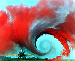
また、自然界に見られるフラクタル構造(シダの葉や雲の形など)は、反復関数系(IFS)というカオス的なプロセスを通じて再現可能です。さらに、生物学的なパターンや、交通流における渋滞の自己組織化、経済市場の変動分析など、広範な分野で応用されています。

![A Conus textile shell, similar in appearance to Rule 30, a cellular automaton with chaotic behaviour[102]](/images/52/a9/52a91a773bd2d573e3b2629dddf8950709173accf54f5c87c4d9e06dfbbed8cb.jpg)
| 概念 | 定義・特徴 | 具体例・現象 |
|---|---|---|
| 初期値鋭敏性 | 微小な差が時間と共に増幅される | 気象予測の限界、二重振り子 |
| ストレンジアトラクター | カオス系が収束する複雑な軌道 | ローレンツ・アトラクター |
| 分岐 (Bifurcation) | パラメータ変化で挙動が劇的に変わること | 周期倍増、ロジスティック写像 |
| フラクタル | 部分が全体と似ている自己相似構造 | バーンズレイのシダ、海岸線 |
Frequently Asked Questions
カオスとランダム(偶然)は何が違うのですか?
ランダムな現象は、根本的に法則性がなく予測不可能なものです。一方、カオスは「決定論的」であり、背後には厳格な数式や法則が存在します。違いは、カオスが初期値に極めて敏感であるため、実質的にランダムに見えるという点にあります。
バタフライ効果は本当に起こるのでしょうか?
物理的な意味で、小さな変化が連鎖的に大きな結果を招くことは多くの非線形システムで確認されています。ただし、あらゆる小さな変化が常に巨大な災害につながるわけではなく、システムがカオス的な状態にある場合にのみ、そのような鋭敏な反応が起こります。
カオス理論を使って未来を予測することはできないのですか?
長期的な予測は不可能ですが、短期的または中期的にはある程度の予測が可能です。また、個別の軌道を予測するのではなく、システムがどのようなアトラクター(構造)を持つかという「統計的な挙動」を把握することで、システムの性質を理解することができます。
どのような分野でカオス理論が活用されていますか?
気象学、流体力学、天文学(三体問題など)といった物理科学から、心拍変動の解析などの生物医学、株価変動の分析などの経済学、さらには暗号技術やロボティクスまで、非常に幅広い分野で活用されています。
References
- "chaos theory | Definition & Facts". Encyclopedia Britannica. Retrieved 2019-11-24.
- "What is Chaos Theory? – Fractal Foundation". Retrieved 2019-11-24.
- Weisstein, Eric W. "Chaos". mathworld.wolfram.com. Retrieved 2019-11-24.
- Boeing, Geoff (26 March 2015). "Chaos Theory and the Logistic Map". Retrieved 2020-05-17.
- Lorenz, Edward (1993). The Essence of Chaos. University of Washington Press. .
- Shen, Bo-Wen; Pielke, Roger A.; Zeng, Xubin; Cui, Jialin; Faghih-Naini, Sara; Paxson, Wei; Atlas, Robert (2022). "Three Kinds of Butterfly Effects within Lorenz Models". Encyclopedia. 2 (3): 1250–1259. :10.3390/encyclopedia2030084. Text was copied from this source, which is available under a Creative Commons Attribution 4.0 International License.
- Kellert, Stephen H. (1993). In the Wake of Chaos: Unpredictable Order in Dynamical Systems. University of Chicago Press. p. 32. .
- Bishop, Robert (2017), "Chaos", in Zalta, Edward N. (ed.), The Stanford Encyclopedia of Philosophy (Spring 2017 ed.), Metaphysics Research Lab, Stanford University, retrieved 2019-11-24
- , p. 56.
- , p. 62.
📸 フォトギャラリー