分子動力学（MD）シミュレーション原子レベルで物質の挙動を解明する計算手法

物質の性質を根本から理解するためには、個々の原子や分子がどのように動き、相互作用しているかを知ることが不可欠です。分子動力学（Molecular Dynamics: MD）は、コンピュータを用いて原子や分子の物理的な動きを解析するシミュレーション手法であり、時間経過に伴うシステムの「進化」を可視化することを可能にします。

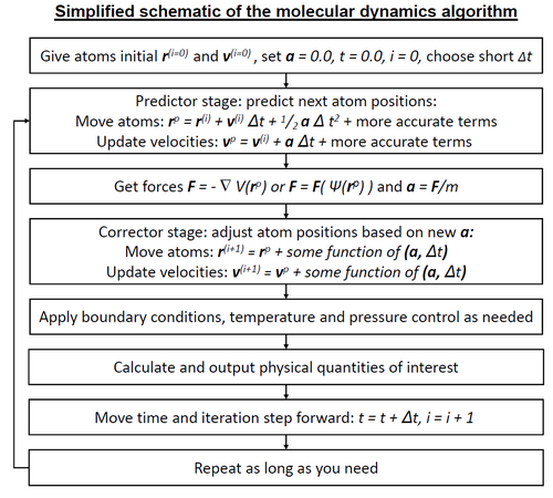
一般的に、MDでは粒子間に働く力とポテンシャルエネルギーを計算し、ニュートンの運動方程式を数値的に解くことで、各粒子の軌道を決定します。この手法は、化学物理学、材料科学、生物物理学など、多岐にわたる分野で不可欠なツールとなっています。

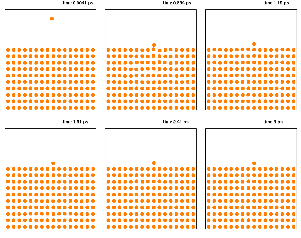
Example of a molecular dynamics simulation in a simple system: deposition of one copper (Cu) atom on a cold crystal of copper (Miller index (001) surface). Each circle represents the position of one atom. The kinetic energy of the atom approaching from the top is redistributed among the other atoms, so instead of bouncing off it remains attached due to attractive forces between the atoms.

Key Facts

基本原理：ニュートンの運動方程式を数値的に解き、原子の軌道を追跡する。
目的：ミクロな原子の動きから、マクロな熱力学的性質を導き出す。
計算手法：古典的な力場（Force Field）から量子力学的な手法まで、多様なポテンシャル関数を利用する。
適用分野：タンパク質の構造解析、新材料の開発、溶媒効果の解析など。
計算コスト：粒子数とシミュレーション時間に比例して増大するため、GPUなどの専用ハードウェアが活用される。

MDシミュレーションの理論的基盤

分子システムは膨大な数の粒子で構成されているため、解析的に（数式だけで）その性質を導き出すことは不可能です。そこでMDは数値計算を用いてこの課題を解決します。ただし、長時間のシミュレーションでは数値積分の累積誤差が発生するため、適切なアルゴリズムの選択が精度維持の鍵となります。

また、システムがエルゴード仮説（十分な時間が経過すれば、時間平均がアンサンブル平均に一致するという考え方）に従う場合、単一のシミュレーション軌跡からマクロな熱力学的性質を推定できます。これはまさに「数値による統計力学」の実践と言えます。

One of the earliest simulations of an N-body system was carried out on the MANIAC-I by Fermi and coworkers to understand the origins of irreversibility in nature. Shown here is the energy versus time for a 64-particle system.

制御される物理的条件（アンサンブル）

シミュレーションの目的に応じて、維持すべき物理量（変数）を定義します。これをアンサンブルと呼びます。

NVEアンサンブル（ミクロカノニカル）：粒子数(N)、体積(V)、エネルギー(E)を一定に保つ。
NVTアンサンブル（カノニカル）：粒子数(N)、体積(V)、温度(T)を一定に保つ。
NPTアンサンブル（等温等圧）：粒子数(N)、圧力(P)、温度(T)を一定に保つ。

ポテンシャルと計算モデルの多様性

原子間にどのような力が働くかを定義するのが「ポテンシャル」です。計算コストと精度のトレードオフにより、以下のような手法が使い分けられます。

経験的ポテンシャルと力場

実験データや理論に基づいた関数を用いて力を近似する手法です。ペアポテンシャル（2粒子間）や多体ポテンシャルがあり、計算負荷が低いため大規模なシステムに適しています。また、電荷の変動を考慮した分極可能ポテンシャルを用いることで、より現実的な挙動を再現できます。

第一原理（Ab Initio）およびハイブリッド手法

量子力学に基づいて電子状態から力を計算する手法です。非常に高精度ですが計算負荷が極めて高く、小規模なシステムに限定されます。これを補うため、重要な部位のみを量子力学で、それ以外を古典力学で計算するQM/MM（量子力学/分子力学）ハイブリッド法も利用されます。

A simplified description of the standard molecular dynamics simulation algorithm, when a predictor-corrector-type integrator is used. The forces may come either from classical interatomic potentials (described mathematically as F = − ∇ V ( r → ) {\displaystyle F=-\nabla V({\vec {r}})} ) or quantum mechanical (described mathematically as F = F ( Ψ ( r → ) ) {\displaystyle F=F(\Psi ({\vec {r}}))} ) methods. Large differences exist between different integrators; some do not have exactly the same highest-order terms as indicated in the flow chart, many also use higher-order time derivatives, and some use both the current and prior time step in variable-time step schemes.

粗視化（Coarse-graining）モデル

複数の原子を一つの「擬似原子」としてまとめることで、計算量を大幅に削減する手法です。例えば、DNAのスーパーコイル構造の解析では、1塩基対あたり1〜3個の擬似原子に簡略化して解析が行われています。

Schematic representation of the sampling of the system's potential energy surface with molecular dynamics (in red) compared to Monte Carlo methods (in blue)

アルゴリズムと計算の最適化

効率的なシミュレーションを実現するためには、高度な数値積分法と計算戦略が必要です。

数値積分法（インテグレータ）

Verlet法やRunge-Kutta法などのアルゴリズムを用いて、時間ステップごとの位置と速度を更新します。特に、エネルギー保存性に優れたシンプレクティック積分法などが重要視されます。

相互作用の計算効率化

すべての粒子ペアを計算すると計算量が膨大になるため、以下の手法が導入されています。

短距離相互作用：セルリストやVerletリストを用いて、近傍の粒子のみを計算対象とする。
長距離相互作用：エバルト和（Ewald summation）やPME（Particle Mesh Ewald）法を用いて、静電相互作用などを効率的に処理する。

Molecular dynamics simulations are often used to study biophysical systems. Depicted here is a 100 ps simulation of water.

ハードウェアの進化

計算速度を向上させるため、ドメイン分解法による並列計算や、GPU（グラフィックスプロセッサ）の活用が進んでいます。また、AntonのようなMD専用の超並列スーパーコンピュータも開発されており、タンパク質の折り畳みなどの長時間現象の解析を可能にしています。

Ionic liquid simulation on GPU (Abalone)

応用事例

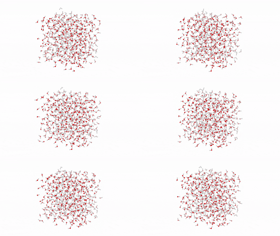
MDシミュレーションは、目に見えないナノスケールの現象を可視化し、予測するために活用されています。

生物物理学：タンパク質の構造予測、リガンドと受容体の相互作用解析、膜透過プロセスの研究。
材料科学：セメント系材料（C-S-Hゲルなど）の弾性特性評価、ナノ結晶アルミニウムの粒成長解析。
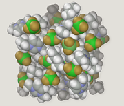
ナノテクノロジー：ナノポア内での合成分子モーターの挙動解析。

Molecular dynamics simulation of a synthetic molecular motor composed of three molecules in a nanopore (outer diameter 6.7 nm) at 250 K[90]

手法	計算コスト	精度	主な適用対象
粗視化モデル	非常に低い	低い（傾向把握）	巨大分子、長時間現象
古典力場 (MD)	低い〜中程度	中程度	タンパク質、液体、ポリマー
第一原理 (Ab Initio)	非常に高い	非常に高い	化学反応、電子状態解析
QM/MM ハイブリッド	中〜高	部位により異なる	酵素反応、活性部位解析

Frequently Asked Questions

MDシミュレーションとモンテカルロ法は何が違うのですか？

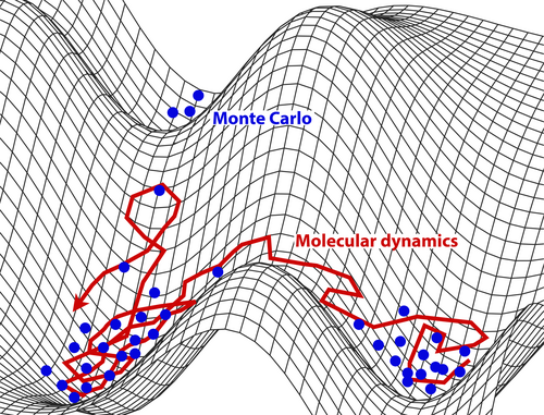
MDはニュートンの運動方程式に基づき、時間の経過に伴う粒子の「軌跡」を追跡する決定論的な手法です。一方、モンテカルロ法は確率的なサンプリングを用いてシステムの平衡状態を探索する手法であり、時間軸の概念を持ちません。

シミュレーション結果の信頼性はどのように担保されますか？

適切な力場の選択、十分なサンプリング時間（平衡化）、および実験値（X線結晶構造解析やNMRなど）との比較検証を行うことで信頼性を担保します。また、数値積分の誤差を最小限に抑えるアルゴリズムの選択も重要です。

なぜGPUがMDシミュレーションに有効なのですか？

MDの計算の大部分は、数多くの粒子ペアに対する相互作用の計算という単純かつ大量の反復処理です。GPUはこのような並列処理に特化したアーキテクチャを持っているため、CPU単体よりも劇的に計算速度を向上させることができます。

機械学習はMDにどのように活用されていますか？

最近では、第一原理計算の精度を維持しつつ、古典力場並みの計算速度を実現する「機械学習力場（MLFF）」の開発が進んでいます。これにより、従来の手法では不可能だった「高精度かつ大規模」なシミュレーションが可能になりつつあります。

References

Abdulhamza HM, Farhan MS, Hassan SS, Aqeel Al-Hussainy H, Oriabi AI (2024). "In silico identification of antiviral compounds for the treatment of chikungunya virus infection: qsar modelling and md simulation analysis". Medicine in Novel Technology and Devices. 22 100304. :10.1016/j.medntd.2024.100304.
Schlick T (1996). "Pursuing Laplace's Vision on Modern Computers". Mathematical Approaches to Biomolecular Structure and Dynamics. The IMA Volumes in Mathematics and its Applications. Vol. 82. pp. 219–247. :10.1007/978-1-4612-4066-2_13. .
Bernal JD (January 1997). "The Bakerian Lecture, 1962 The structure of liquids". Proceedings of the Royal Society of London. Series A. Mathematical and Physical Sciences. 280 (1382): 299–322. :1964RSPSA.280..299B. :10.1098/rspa.1964.0147. 178710030.
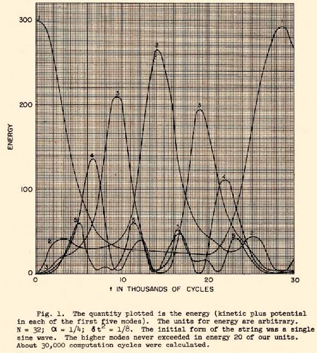
Fermi E., Pasta J., Ulam S., Los Alamos report LA-1940 (1955).
Alder BJ, Wainwright T (August 1959). "Studies in Molecular Dynamics. I. General Method". The Journal of Chemical Physics. 31 (2): 459–466. :1959JChPh..31..459A. :10.1063/1.1730376.
Gibson JB, Goland AN, Milgram M, Vineyard G (1960). "Dynamics of Radiation Damage". Phys. Rev. 120 (4): 1229–1253. :1960PhRv..120.1229G. :10.1103/PhysRev.120.1229.
(19 October 1964). "Correlations in the Motion of Atoms in Liquid Argon". Physical Review. 136 (2A): A405–A411. :1964PhRv..136..405R. :10.1103/PhysRev.136.A405.
Stephan S, Thol M, Vrabec J, Hasse H (October 2019). "Thermophysical Properties of the Lennard-Jones Fluid: Database and Data Assessment". Journal of Chemical Information and Modeling. 59 (10): 4248–4265. :10.1021/acs.jcim.9b00620. 31609113. 204545481.
Wang X, Ramírez-Hinestrosa S, Dobnikar J, Frenkel D (May 2020). "The Lennard-Jones potential: when (not) to use it". Physical Chemistry Chemical Physics. 22 (19): 10624–10633. :1910.05746. :2020PCCP...2210624W. :10.1039/C9CP05445F. 31681941. 204512243.
Mick J, Hailat E, Russo V, Rushaidat K, Schwiebert L, Potoff J (December 2013). "GPU-accelerated Gibbs ensemble Monte Carlo simulations of Lennard-Jonesium". Computer Physics Communications. 184 (12): 2662–2669. :2013CoPhC.184.2662M. :10.1016/j.cpc.2013.06.020.