多変数関数を扱う解析学において、勾配(グラディエント)は関数の変化をベクトルとして表現する極めて重要な概念です。ある点における関数の値がどの方向に、どれだけの速さで変化するかを定量的に示すことで、物理学から最適化問題まで幅広い分野で活用されています。
Key Facts
- 勾配は、スカラー関数からベクトル場を生成する演算である。
- ベクトルとしての方向は、関数値が最も急激に増加する方向(最急上昇方向)を指す。
- 各成分は、それぞれの座標軸方向への偏微分によって構成される。
- 等高線(レベルセット)に対して常に直交する性質を持つ。
- 内積を用いることで、任意の方向への変化率(方向微分)を算出できる。
勾配の基礎概念と定義
勾配とは、ある点におけるスカラー関数 $f$ の変化率をベクトル形式でまとめたものです。数学的には、ベクトル微分演算子であるナブラ ($\nabla$) を用いて $\nabla f$ または $\text{grad } f$ と表記されます。
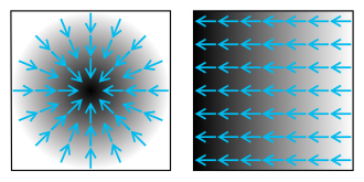
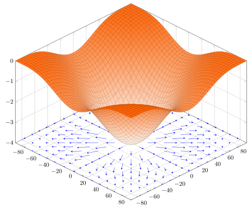
直感的に説明すると、山のような地形(スカラー場)において、ある地点から見て「最も急な上り坂」の方向と、その傾斜の強さを一つの矢印で表したものが勾配に相当します。
数学的な定義
勾配は、任意の単位ベクトル $\mathbf{v}$ との内積をとったとき、その方向への方向微分 $D_{\mathbf{v}}f(x)$ と一致する唯一のベクトル場として定義されます。数式では以下のように表されます: $(\nabla f(x)) \cdot \hat{\mathbf{v}} = D_{\mathbf{v}}f(x)$
座標系による計算方法
勾配の具体的な計算方法は、使用する座標系によって異なります。
デカルト座標系(直交座標系)
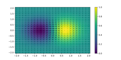
3次元のデカルト座標系では、各軸方向の偏微分を成分とするベクトルとして求められます。関数 $f(x, y, z)$ の勾配は以下の通りです: $\nabla f = \frac{\partial f}{\partial x}\mathbf{i} + \frac{\partial f}{\partial y}\mathbf{j} + \frac{\partial f}{\partial z}\mathbf{k}$
円筒座標系と球座標系
曲面や回転体を扱う場合、以下の座標系が便利です。
- 円筒座標系 $(\rho, \varphi, z)$: $\nabla f = \frac{\partial f}{\partial \rho}\mathbf{e}_\rho + \frac{1}{\rho}\frac{\partial f}{\partial \varphi}\mathbf{e}_\varphi + \frac{\partial f}{\partial z}\mathbf{e}_z$
- 球座標系 $(r, \theta, \varphi)$: $\nabla f = \frac{\partial f}{\partial r}\mathbf{e}_r + \frac{1}{r}\frac{\partial f}{\partial \theta}\mathbf{e}_\theta + \frac{1}{r\sin\theta}\frac{\partial f}{\partial \varphi}\mathbf{e}_\varphi$
勾配の性質と応用
最急上昇方向と方向微分
勾配ベクトル $\nabla f$ は、関数値が最大速度で増加する方向を指します。一方で、勾配方向とは異なる任意の方向への傾斜を知りたい場合は、勾配ベクトルと方向単位ベクトルの内積を計算します。例えば、最急上昇方向から60度の角度にある道を進む場合、その方向の傾斜は「最急傾斜 $\times \cos(60^\circ)$」となり、元の傾斜の半分になります。
線形近似への利用
ある点 $x_0$ の近傍において、関数 $f(x)$ は勾配を用いて以下のように線形近似(一次近似)することが可能です: $f(x) \approx f(x_0) + (\nabla f)_{x_0} \cdot (x - x_0)$ これは多変数関数のテイラー展開の最初の2項に相当します。
レベルセット(等値面)との関係
関数 $F(x_1, \dots, x_n) = 0$ で定義される超曲面において、勾配 $\nabla F$ はその点における法線ベクトル(面に垂直なベクトル)となります。勾配がゼロになる点は、その曲面の特異点として定義されます。
高度な一般化
ヤコビ行列への拡張
スカラー関数ではなく、ベクトル値関数 $\mathbf{f}: \mathbb{R}^n \to \mathbb{R}^m$ の場合、各成分関数の勾配を並べたヤコビ行列 $\mathbf{J}$ として一般化されます。これは多変数関数の微分を行列形式で表現したものです。
リーマン多様体における勾配
曲がった空間(リーマン多様体)では、計量テンソル $g$ を用いて勾配が定義されます。任意のベクトル場 $X$ に対して $g(\nabla f, X) = \partial_X f$ を満たすベクトル場 $\nabla f$ が勾配となります。局所座標では $\nabla f = g^{ik} \frac{\partial f}{\partial x^k} \mathbf{e}_i$ と記述されます。
まとめ:勾配の特性一覧
| 特性 | 内容 | 数学的意味 |
|---|---|---|
| 方向 | 関数値が最も速く増加する方向 | 最急上昇方向 |
| 大きさ | その方向への最大変化率 | $||\nabla f||$ |
| 幾何学的関係 | 等高線(レベルセット)に直交する | 法線ベクトル |
| 演算 | 偏微分のベクトル合成 | $\nabla f = [\partial f/\partial x_1, \dots, \partial f/\partial x_n]^T$ |
Frequently Asked Questions
勾配と全微分はどう違うのですか?
全微分 $df$ は通常、行ベクトル(または線形写像)として表現され、関数値の変化量を表します。一方、勾配 $\nabla f$ は列ベクトルとして表現され、ユークリッド空間における「方向」と「大きさ」を持つベクトルとして定義されます。標準的な計量の下では、全微分の転置が勾配に相当します。
なぜ勾配は最急上昇方向を指すのですか?
方向微分は勾配ベクトルと方向単位ベクトルの内積で求められます。内積の性質上、2つのベクトルが同じ方向を向いているときに値が最大となるため、勾配ベクトル自身の方向が最大変化率(最急上昇)を与える方向になります。
偏微分ができれば必ず勾配が存在しますか?
いいえ。すべての方向への偏微分が存在していても、関数がその点で微分可能(接平面が適切に定義されている状態)でない場合があります。そのような場合、単純な偏微分の組み合わせではベクトルとして正しく変換されず、最急上昇方向を正しく指し示さないことがあります。
勾配がゼロであることは何を意味しますか?
勾配がゼロの点は「臨界点」と呼ばれます。これは、関数が極大値、極小値、あるいは鞍点(サドルポイント)にある可能性を示しており、最適化問題において解を探索する際の重要な指標となります。
References
- This article uses the convention that represent vectors, and represent covectors, but the opposite convention is also common.
- Strictly speaking, the gradient is a , and the value of the gradient at a point is a in the at that point, , not a vector in the original space . However, all the tangent spaces can be naturally identified with the original space , so these do not need to be distinguished; see and .
- The value of the gradient at a point can be thought of as a vector in the original space , while the value of the derivative at a point can be thought of as a covector on the original space: a linear map .
- the dot product (the slope of the road around the hill) would be 40% if the degree between the road and the steepest slope is 0°, i.e. when they are completely aligned, and flat when the degree is 90°, i.e. when the road is perpendicular to the steepest slope.
- Informally, "naturally" identified means that this can be done without making any arbitrary choices. This can be formalized with a .
 , and the value of the gradient at a point is a in the at that point,
  , not a vector in the original space
  . However, all the tangent spaces can be naturally identified with the original space
  .
.📸 フォトギャラリー