数学の世界において、リーマンゼータ関数($\\zeta(s)$)は、数論の根幹を支える極めて重要な関数です。一見すると単純な無限級数の形をしていますが、その性質は素数の出現パターンという、数学における最大の謎の一つと深く結びついています。物理学や確率論、統計学など、純粋数学の枠を超えて幅広い分野で応用されているこの関数について解説します。
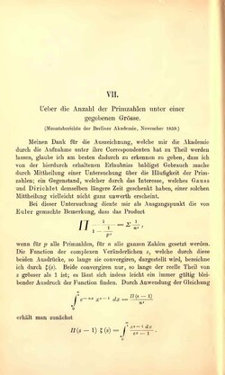
もともと18世紀前半にレオンハルト・オイラーが実数範囲で研究していましたが、1859年にベルンハルト・リーマンがこれを複素数へと拡張しました。リーマンは、関数の「零点(値が0になる点)」の分布が、素数の分布を決定づけることを突き止め、現代の解析数論の扉を開いたのです。
Key Facts
- 定義: 実部が1より大きい複素数 $s$ に対して $\\zeta(s) = \\sum_{n=1}^{\\infty} n^{-s}$ と定義され、その後解析接続によって領域を広げている。
- 素数との関係: オイラー積と呼ばれる公式により、すべての素数の積として表現できる。
- リーマン予想: 「非自明な零点はすべて実部が1/2の直線(臨界線)上にある」という、数学史上最も重要な未解決問題の一つ。
- 応用範囲: 解析数論だけでなく、量子力学などの物理学や統計学にも影響を与えている。
ゼータ関数の基礎と定義
リーマンゼータ関数は、複素変数 $s$ を用いて以下のように定義されます。まず、実部 $\\text{Re}(s) > 1$ の範囲では、自然数のべき乗の逆数の和として表されます。
この定義を、解析接続(ある領域で定義された関数を、その性質を保ったまま別の領域へ拡張する手法)を用いることで、$s=1$(極)を除く複素平面全体に広げることができます。
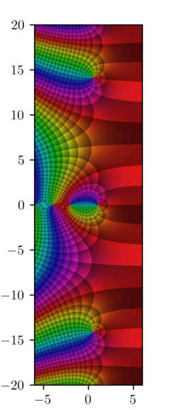
![The Riemann zeta function ζ(z) plotted with domain coloring[1]](/images/dd/c0/ddc018df078b3b066807db5e5d73b0a32c10c6c431be4a28258935e6d6f42fee.webp)
オイラー積:素数への架け橋
1737年、オイラーはゼータ関数がすべての素数 $p$ を用いた無限積で書き換えられることを証明しました。これにより、ゼータ関数を解析することで、不規則に見える素数の分布を数学的に扱えることが明らかになりました。
零点とリーマン予想
ゼータ関数が0になる点(零点)には、2つの種類があります。一つは負の偶数(-2, -4, ...)に現れる「自明な零点」であり、もう一つは複素平面上の特定の帯状領域(臨界帯)に現れる「非自明な零点」です。
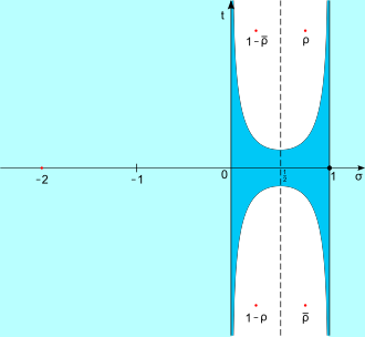
リーマンは、これらの非自明な零点がすべて臨界線(実部が1/2の直線)上に並んでいるのではないかという大胆な予想を立てました。これが有名な「リーマン予想」です。もしこれが正しければ、素数の分布に関する誤差が極めて小さく抑えられていることが証明されます。
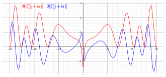
臨界線上の挙動
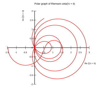
計算機による検証では、数兆個以上の零点がすべてこの臨界線上に存在することが確認されています。また、零点の虚部は $\\pm 14.135, \\pm 21.022, \\pm 25.011$ といった値をとることが知られています。
数学的特性と表現形式
ゼータ関数は、その用途に応じてさまざまな形式で表現されます。例えば、ガンマ関数を用いた関数等式や、メリン変換による積分表示、あるいはヤコビのテータ関数を用いた表現などが存在します。
また、メビウス関数 $\\mu(n)$ を用いたディリクレ級数として、ゼータ関数の逆数 $\\frac{1}{\\zeta(s)}$ を表現することも可能です。これにより、数論的な性質をより深く解析することができます。
| 項目 | 内容・特徴 | 数学的意義 |
|---|---|---|
| 定義域 | 複素平面全体($s=1$ を除く) | 解析接続による拡張 |
| オイラー積 | 素数 $p$ の無限積形式 | 素数分布との直接的な結合 |
| 自明な零点 | $-2, -4, -6, \dots$ | 関数等式から導かれる点 |
| 非自明な零点 | 実部 $0 < \\text{Re}(s) < 1$ の範囲 | リーマン予想の核心部分 |
| 臨界線 | $\\text{Re}(s) = 1/2$ | 零点が集中すると予想される線 |
Frequently Asked Questions
リーマン予想が証明されると何が嬉しいのですか?
素数の分布が極めて正確に把握できるようになります。多くの現代数学の定理が「リーマン予想が正しいと仮定すれば」という前提で構築されており、証明されればそれらの定理がすべて確定的な事実となります。
「解析接続」とは簡単に言うと何ですか?
ある範囲でしか定義できなかった関数を、数学的な整合性を保ったまま、より広い範囲で定義し直す操作のことです。ゼータ関数の場合、もともと $\\text{Re}(s) > 1$ でしか計算できなかった和を、複素平面全体で扱えるようにしています。
自明な零点と非自明な零点の違いは何ですか?
自明な零点は、関数の構造(関数等式)から機械的に導き出される点です。一方、非自明な零点は、その位置が素数の分布という深い数論的性質に依存しており、予測が困難であるため「非自明」と呼ばれます。
ゼータ関数は実生活に役立っているのですか?
直接的な計算で使われることは少ないですが、暗号理論の基礎となる素数論を支えています。また、量子力学におけるエネルギー準位の分布など、物理現象の解析にゼータ関数の性質が応用される事例があります。
References
- "Jupyter Notebook Viewer". Nbviewer.ipython.org. Retrieved 4 January 2017.
- Steuding, Jörn; Suriajaya, Ade Irma (1 November 2020). "Value-Distribution of the Riemann Zeta-Function Along Its Julia Lines". Computational Methods and Function Theory. 20 (3): 389–401. :2007.14661. :10.1007/s40315-020-00316-x. :2324/4483207. 2195-3724. 216323223.
Theorem 2 implies that ζ has an essential singularity at infinity
- Bombieri, Enrico. "The Riemann Hypothesis – official problem description" (PDF). . Archived from the original (PDF) on 22 December 2015. Retrieved 8 August 2014.
- (2002). The Millennium Problems: The seven greatest unsolved mathematical puzzles of our time. New York: Barnes & Noble. pp. 43–47. .
- Sandifer, Charles Edward (2007). How Euler Did It. Mathematical Association of America. p. 193. .
- Mollin, Richard A. (2010). Advanced Number Theory with Applications. Discrete Mathematics and its Applications (Boca Raton). CRC Press, Boca Raton, FL. p. 220. . 2560324.
- Damm-Johnsenn, Håvard (2019). Theta functions and their applications (PDF). p. 5. Archived from the original (PDF) on 21 March 2025.
- Titchmarsh, E.C. (1986). The Theory of the Riemann Zeta Function (2nd ed.). , UK: Oxford Science Publications. pp. 21–22. .
- (1989). "More than two fifths of the zeros of the Riemann zeta function are on the critical line". J. Reine Angew. Math. 1989 (399): 1–26. :10.1515/crll.1989.399.1. 1004130. 115910600.
- Pratt, Kyle; Robles, Nicolas; Zaharescu, Alexandru; Zeindler, Dirk (2020). "More than five-twelfths of the zeros of are on the critical line". Research in the Mathematical Sciences. 7. :1802.10521. :10.1007/s40687-019-0199-8.
 are on the critical line"
📸 フォトギャラリー