線形回帰分析の基礎から応用までデータ間の関係性を解き明かす統計手法

私たちは日常的に、「ある数値が上がれば、別の数値も上がる」といった傾向を分析しています。統計学において、このような変数間の直線的な関係を数式でモデル化する手法が線形回帰分析です。この手法は、単なるデータの傾向把握にとどまらず、将来の予測や要因分析など、科学から経済学、機械学習に至るまで極めて幅広い分野で活用されています。

Key Facts

• 線形回帰は、従属変数（目的変数）と独立変数（説明変数）の間に直線的な関係を想定するモデルである。
• 最小二乗法は、実際のデータ点と回帰直線との誤差の二乗和を最小にするパラメータを求める代表的な推定手法である。
• 単回帰は独立変数が1つ、重回帰は複数の独立変数を用いる。
• 一般化線形モデル (GLM)を用いることで、正規分布以外のデータ（二値データやカウントデータなど）にも対応可能となる。
• 回帰分析の概念は、フランシス・ゴルトンが提唱した「平均への回帰」という現象に由来している。

線形回帰の基本構造と仕組み

線形回帰の核心は、観測されたデータが「ある基本的な直線関係」と、そこから外れる「ランダムなノイズ（誤差）」の組み合わせで構成されていると考える点にあります。数学的には、従属変数 $y$ を、独立変数 $x$ と係数 $\beta$、そして誤差項 $\varepsilon$ を用いて表現します。

例えば、1つの独立変数を用いる単回帰分析では、シンプルな直線の方程式で関係性を記述します。

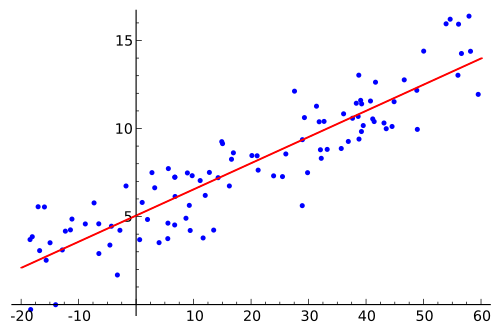
しかし、現実のデータは完璧な直線上に並ぶことはありません。そこで、理論上の直線から実際の観測値がどれだけ離れているかを示す「偏差」を考慮し、モデルを構築します。

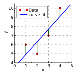
モデルの定式化

複数の独立変数（$x_1, x_2, \dots, x_p$）を持つ重回帰分析の場合、モデルはより複雑な形式になります。行列表記を用いることで、大量のデータセットを効率的に処理することが可能です。このとき、各変数に割り当てられる係数 $\beta$ が、その変数が目的変数に与える影響力の強さを表します。

推定手法とモデルの最適化

モデルを構築する際、最も重要なのは「どの直線（または平面）が最もデータに適合しているか」を決定することです。

最小二乗法 (OLS)

最も一般的な手法が最小二乗法 (Ordinary Least Squares) です。これは、実測値と予測値の差（残差）を二乗し、その合計が最小になるように係数を決定する方法です。また、データの分布がガウス分布（正規分布）に従うと仮定した場合、この手法は最大尤度推定法と一致します。

その他の推定アプローチ

データの特性に応じて、以下のような高度な手法が使い分けられます。

• 重み付き最小二乗法: データの信頼度に差がある場合に、特定のデータに重みを付けて計算します。
• リッジ回帰・Lasso回帰: 正則化という手法を用いて、係数が大きくなりすぎる（過学習する）のを防ぎます。
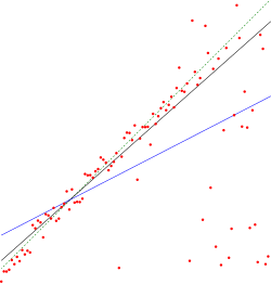
• テイル・セン推定法: 外れ値の影響を受けにくい頑健（ロバスト）な推定が可能です。

回帰分析における注意点と拡張概念

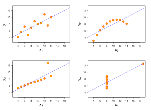
数値的な指標（相関係数や決定係数）だけを信じることは危険です。統計的な数値が似ていても、データの視覚的な分布が全く異なるケースがあるため、必ず散布図などでデータの形状を確認する必要があります。

一般化線形モデル (GLM) への展開

線形回帰は強力ですが、「目的変数が0か1の二値である」場合や「回数がカウントデータである」場合には適用できません。そこで、リンク関数を導入して正規分布以外の分布（二項分布やポアソン分布など）に対応させたのが一般化線形モデルです。これにより、ロジスティック回帰などの高度な分析が可能になります。

歴史的背景：平均への回帰

「回帰 (Regression)」という言葉は、19世紀にフランシス・ゴルトンが親子の身長の関係を研究した際に使われました。極端に身長が高い親を持つ子供であっても、その身長は親よりは平均値に近づく傾向があることが分かり、これが「平均への回帰」と呼ばれたことが現在の名称の由来となっています。

線形回帰のまとめ

線形回帰分析の主要手法比較

手法名	特徴	主な用途
単回帰分析	1つの説明変数で予測	単純な因果関係の把握
重回帰分析	複数の説明変数で予測	複雑な要因分析、精度向上
ロジスティック回帰	目的変数がカテゴリカル（二値）	合格/不合格、発症/未発症の予測
正則化回帰 (Ridge/Lasso)	係数にペナルティを課す	多重共線性への対策、変数選択

Frequently Asked Questions

線形回帰と相関分析の違いは何ですか？

相関分析は2つの変数の「連動性の強さ」を測るもので、どちらが原因でどちらが結果かは問いません。一方、線形回帰は「独立変数が従属変数にどのような影響を与えるか」という因果関係を数式化し、予測を行うことを目的としています。

外れ値がある場合はどうすればよいですか？

通常の最小二乗法は外れ値に非常に敏感で、結果が大きく歪むことがあります。その場合は、外れ値の影響を抑えることができるロバスト回帰や、テイル・セン推定法などの代替手法を検討することが推奨されます。

「多重共線性」とは何ですか？

重回帰分析において、独立変数同士が強く相関している状態を指します。これにより係数の推定が不安定になり、正しく解釈できなくなることがあります。対策として、変数の削除や主成分分析による次元圧縮、あるいはリッジ回帰などの正則化手法が用いられます。

線形回帰を適用するための前提条件はありますか？

一般的に、誤差項が独立であること、等分散性（分散が一定であること）、および誤差項が正規分布に従うことが前提とされます。これらの仮定が崩れている場合は、重み付き最小二乗法や一般化線形モデルへの移行を検討します。

References

- (2009). Statistical Models: Theory and Practice. . p. 26.
A simple regression equation has on the right hand side an intercept and an explanatory variable with a slope coefficient. A multiple regression e right hand side, each with its own slope coefficient
- Rencher, Alvin C.; Christensen, William F. (2012), "Chapter 10, Multivariate regression – Section 10.1, Introduction", Methods of Multivariate Analysis, Wiley Series in Probability and Statistics, vol. 709 (3rd ed.), John Wiley & Sons, p. 19, , archived from the original on 2024-10-04, retrieved 2015-02-07.
- "Linear Regression in Machine learning". GeeksforGeeks. 2018-09-13. Archived from the original on 2024-10-04. Retrieved 2024-08-25.
- Yan, Xin (2009), Linear Regression Analysis: Theory and Computing, World Scientific, pp. 1–2, , archived from the original on 2024-10-04, retrieved 2015-02-07,
Regression analysis ... is probably one of the oldest topics in mathematical statistics dating back to about two hundred years ago. The earliest form of the linear regression was the least squares method, which was published by Legendre in 1805, and by Gauss in 1809 ... Legendre and Gauss both applied the method to the problem of determining, from astronomical observations, the orbits of bodies about the sun.
- Romano, Joseph P.; Wolf, Michael (2017). "Resurrecting weighted least squares". . 197 (1). Elsevier: 1–19. :10.1016/j.jeconom.2016.10.003.
- Berk, Richard A. (2007). "Regression Analysis: A Constructive Critique". Criminal Justice Review. 32 (3): 301–302. :10.1177/0734016807304871. 145389362.
- Hidalgo, Bertha; (2012-11-15). "Multivariate or Multivariable Regression?". American Journal of Public Health. 103 (1): 39–40. :10.2105/AJPH.2012.300897. 0090-0036. 3518362. 23153131.
- Brillinger, David R. (1977). "The Identification of a Particular Nonlinear Time Series System". Biometrika. 64 (3): 509–515. :10.1093/biomet/64.3.509. 2345326.
- Tsao, Min (2022). "Group least squares regression for linear models with strongly correlated predictor variables". Annals of the Institute of Statistical Mathematics. 75 (2): 233–250. :1804.02499. :10.1007/s10463-022-00841-7. 237396158.
- Galton, Francis (1886). "Regression Towards Mediocrity in Hereditary Stature". The Journal of the Anthropological Institute of Great Britain and Ireland. 15: 246–263. :10.2307/2841583. 0959-5295. 2841583.